

Transformationen bestehen aus Gleichungen und Funktionen in der SigmaPlot
Transforms-Sprache. Sie führen Berechnungen und Datenanalyse aus.
Die Datei Xfms.jnb enthält in 55 Sections Beispiele von SigmaPlot User-Defined Transforms. Sie finden die Datei im Help-Menü > Samples > "Transforms" (* -> neu in v14).
Die meisten der Beispiele in dieser Datei haben auch eine Graphseite
mit einem vorbereiteten Graphen.
Aus den Rohwerten im Arbeitsblatt berechnet die Transformation die Daten,
die dann im Graphen dargestellt werden.
Graphen und Kommentarblöcke der Transformationen werden in der unteren Tabelle
auf dieser Seite angezeigt.
 (ToolTip)
| Description | Notebook Section | |
|---|---|---|
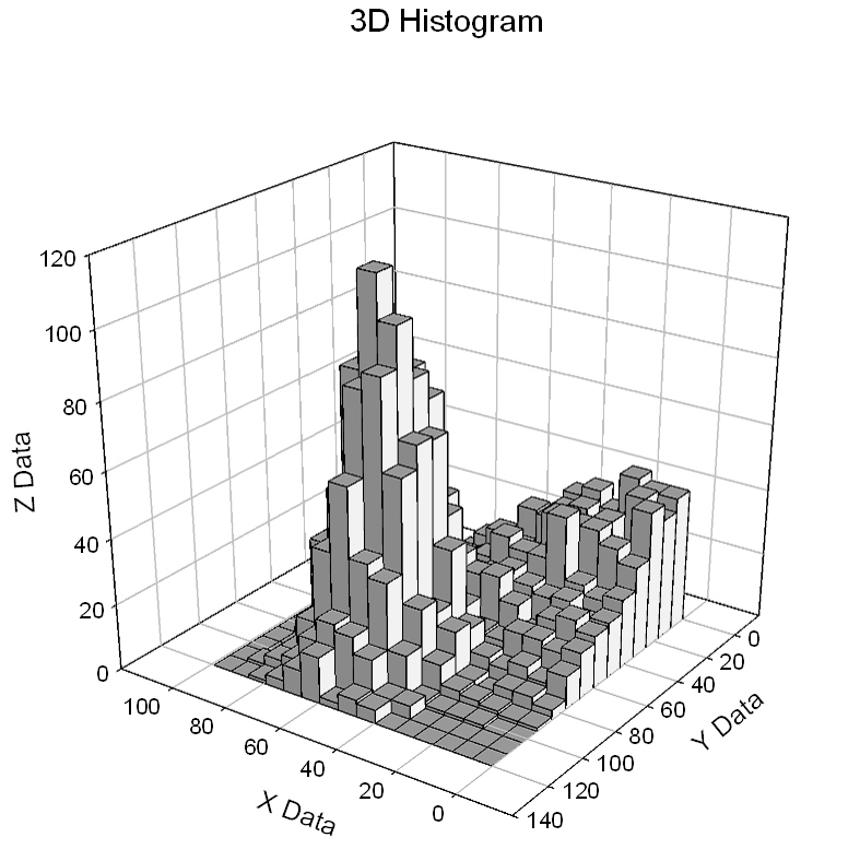
| 3D Histogram * |
|
3D Histogram |
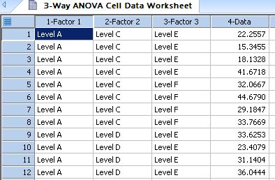
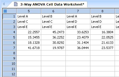
| Converts indexed data for a 3-Way ANOVA design into a raw data format * |
|
3-Way ANOVA Cell Data |
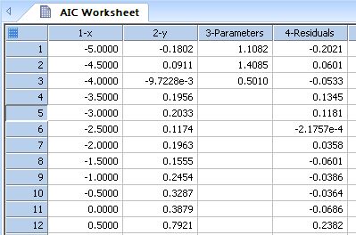
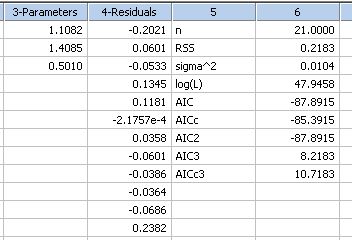
| Akaike Information Criteria - Model Comparisons * |
|
Akaike Information Criteria |
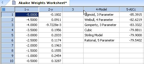
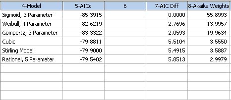
| Akaike Model Probabilities * |
|
Akaike Weights |
| Transform for Calculating Area Beneath a Curve |
|
Area Under Curve |
| Transform to Compute Bivariate Statistics |
|
Bivariate Data Analysis |
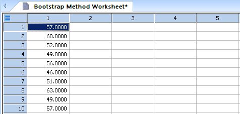
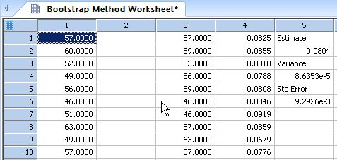
| Bootstrapping to Estimate Variance of a Statistic * |
|
Bootstrap Method |
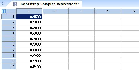
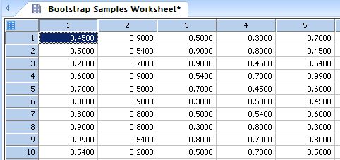
| Creates a number of bootstrap samples (sampling with replacement) of a user-selected column of worksheet data * |
|
Bootstrap Samples |
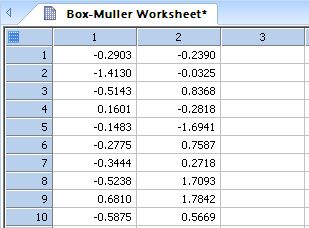
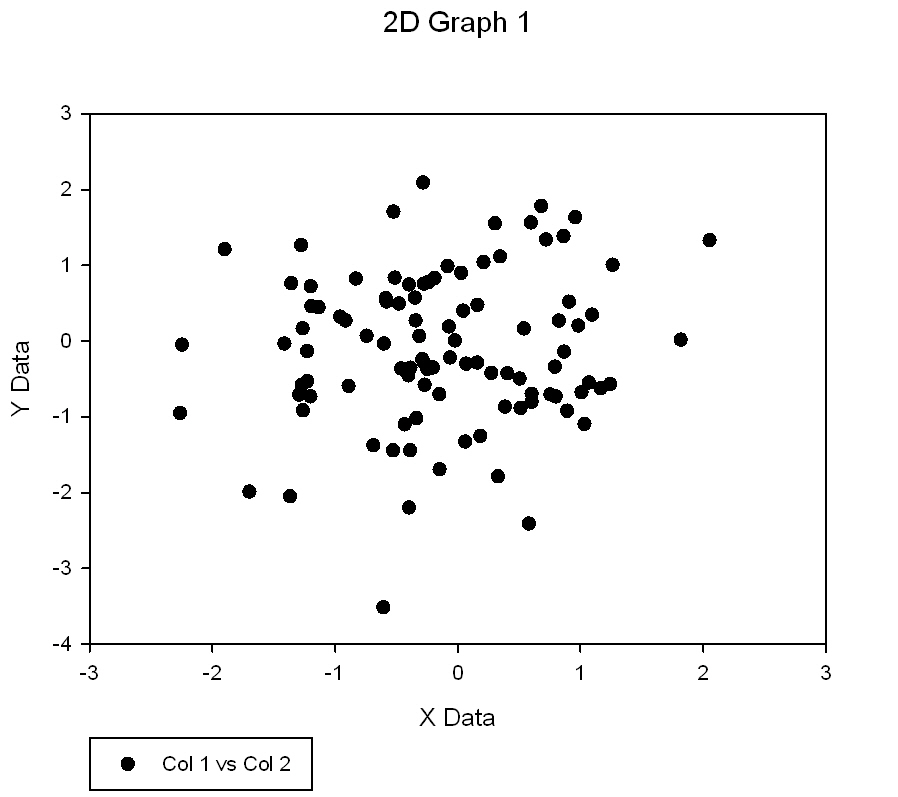
| Box and Mullers Bivariate Normal Random Number Generator * |
|
Box-Muller Bivariate Normal Deviates |
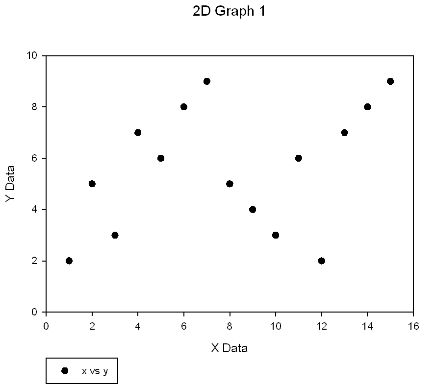
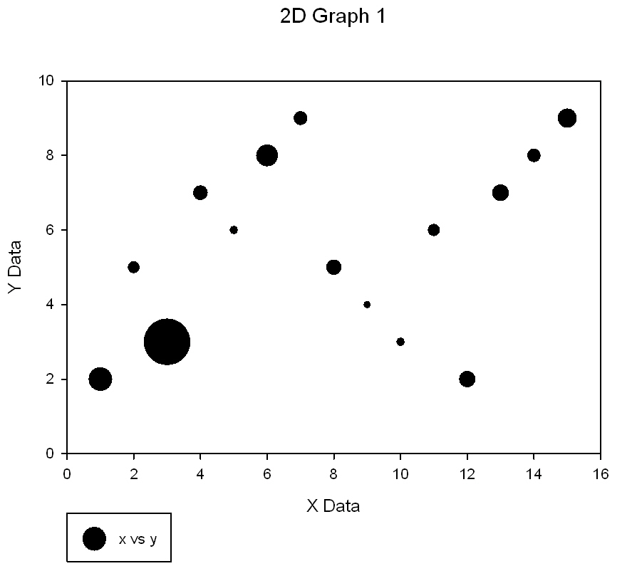
| Symbol Size for Bubble Plot (Symbol Sizexfm) |
|
Bubble Plot Symbol Size |
| Transform for Fraction Defective Control Chart with Unequal Sample Sizes |
|
Control Chart |
| Convert data from Cartesian coordinates to Polar coordinates * |
|
Convert Cartesian To Polar |
| Convert data from Polar coordinates to Cartesian coordinates * |
|
Convert Polar To Cartesian |
| Vector Plot Conversion XYAM to XYXY * |
|
Convert Vector Plot Data Formats |
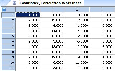
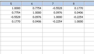
| Computes the sample covariance matrix or the sample correlation matrix of multivariate data * |
|
Covariance_Correlation Matrix |
| Cubic Spline Interpolation and Computation of Derivatives |
|
Cubic Spline |
| D'Agostino-Pearson Normality Test * |
|
D'Agostino-Pearson Normality Test |
| Solution of Coupled First Order Differential Equations by Fourth Order Runge-Kutta Method * |
|
Differential Equation - Runge Kutta |
| Procedure to locate all weak, local maxima or minima in a data set * |
|
Extrema Locator |
| This transform creates frequency plots and mean bars of multiple y data columns |
|
Frequency Plot |
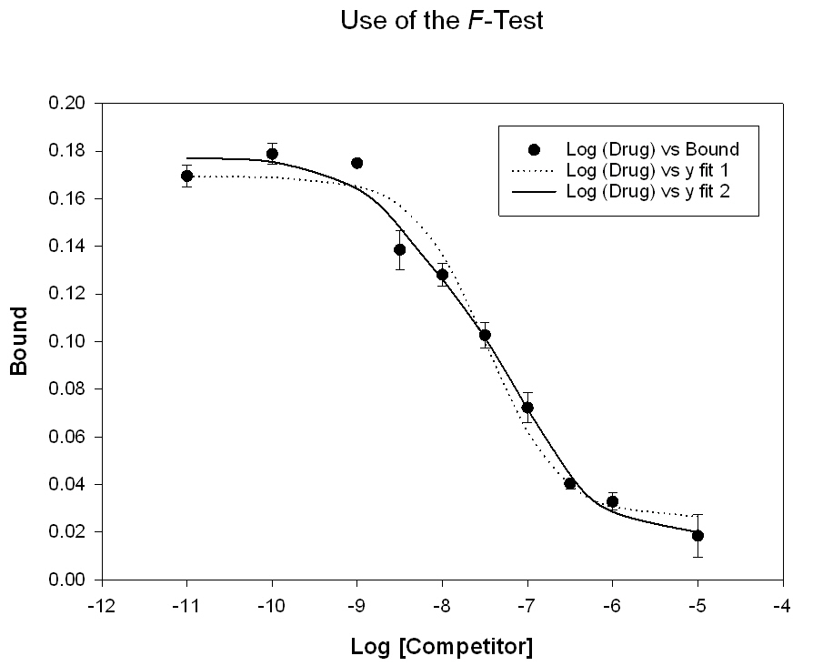
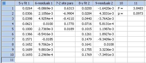
| Compare Two Nonlinear Curve Fits with the F test |
|
F-Test |
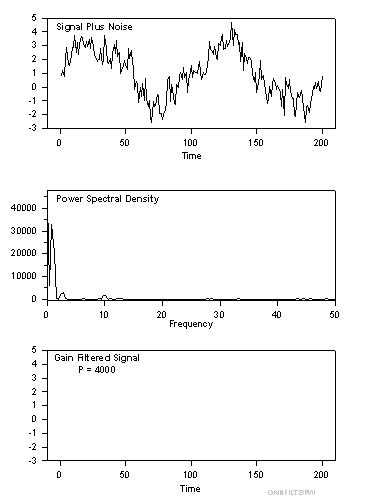
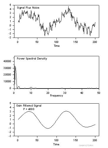
| Gain Filtering |
|
Gain Filter Smoothing |
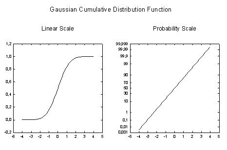
| Gaussian Cumulative Distribution Function |
|
Gaussian |
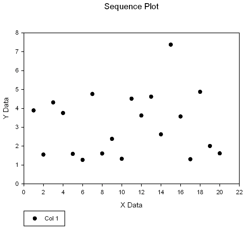
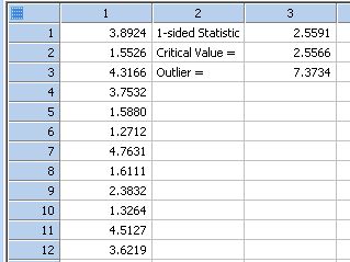
| Grubbs' Single-Outlier Test ( Maximum Normed Residual Test) * |
|
Grubbs' Single-Outlier Test |
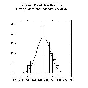
| Transform for a Histogram with a Superimposed Gaussian Distribution |
|
Histogram Gaussian |
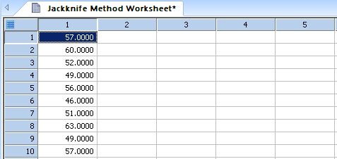
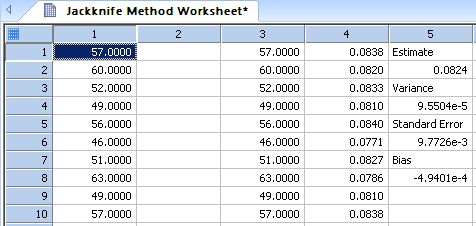
| Jackknife Method to Estimate Variance of a Statistic * |
|
Jackknife Method |
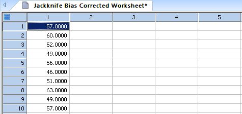
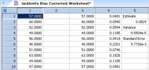
| Jackknife Method with Bias Correction to Estimate Variance of a Statistic * |
|
Jackknife Method - Bias Corrected |
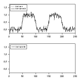
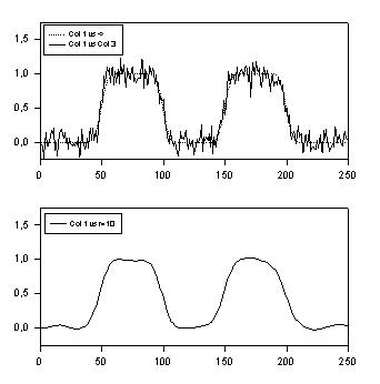
| This transform smooths data using kernel smoothing |
|
Kernel Smoothing |
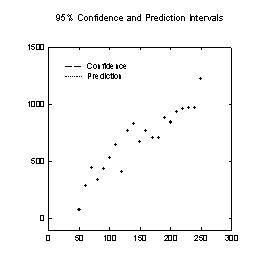
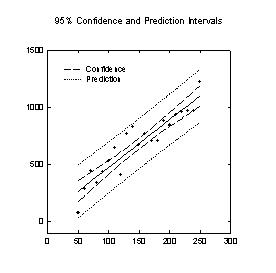
| Transform to Compute a Linear Regression with Confidence & Prediction Intervals |
|
Linear Regression |
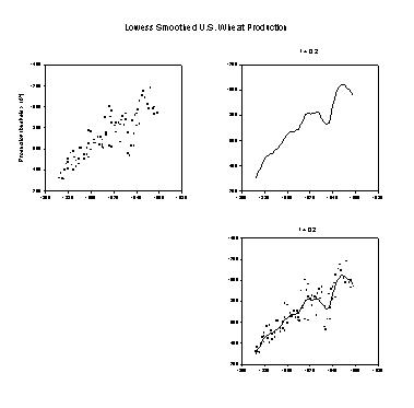
| Lowess Smoothing Example |
|
Lowess Smoothing |
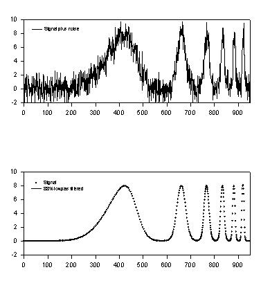
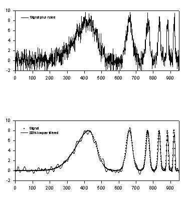
| Lowpass Smoothing Filter |
|
Low Pass Smoothing |
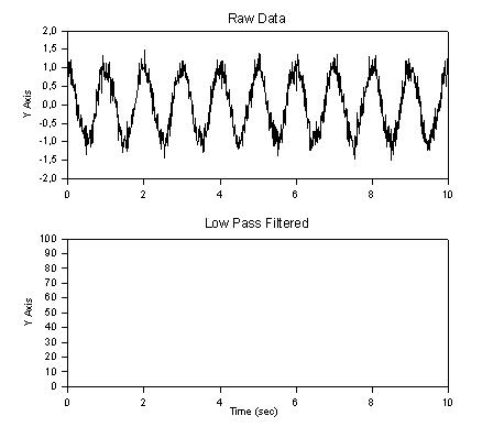
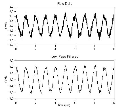
| First Order Low Pass Recursive Filter |
|
Low Pass Filter |
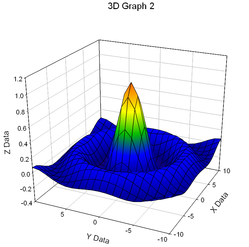
| Transform to generate XYZ triplet data for Mesh Graph |

|
Mesh Plot |
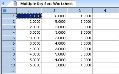
| Performs an in-place sort of a block of data in the worksheet with multiple key columns * |

|
Multiple Key Sort |
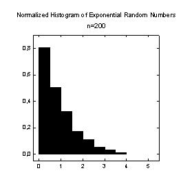
| Transform to Generate Normalized Histogram |
|
Normalized Histogram |
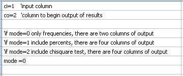
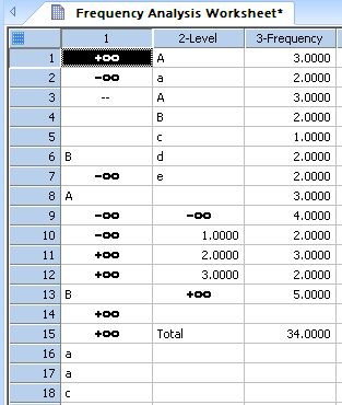
| This transform will find the unique items in the input column and give the count or frequency of each item in the column * |
|
One-Way Frequency Analysis |
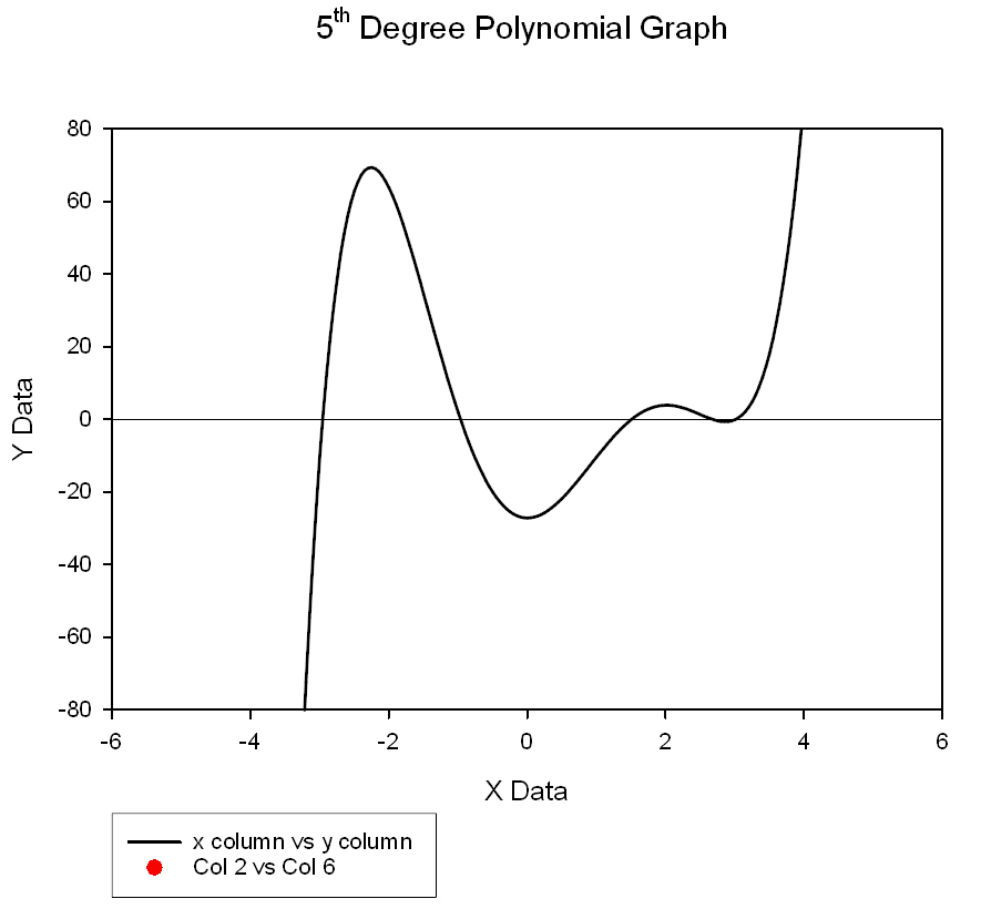
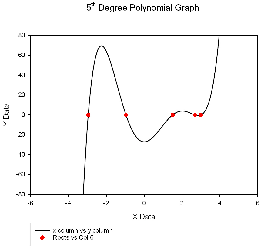
| This transform computes the real roots (zeroes) of a polynomial with real coefficients. * |
|
Polynomial Roots |
| This transform computes the power spectral density (psd) of the data in column ci and places it in column co |
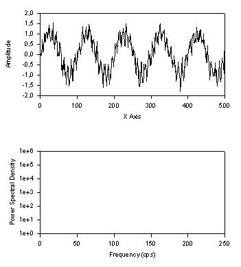
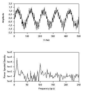
|
Power Spectral Density |
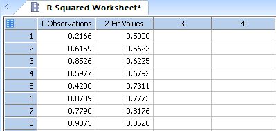
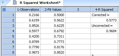
| Transform to Compute R Square (Coefficient of Determination) for Non-linear Curve Fits |
|
R Squared |
| Generates random numbers with a given distribution determined by the user. |
|
Random numbers, Assorted Distributions |
| This transform takes x,y and multiple z columns and creates x,y,z ribbon triplets |
|
Ribbon Plot Data |
| Rosner's Generalized ESD Multiple Outlier Procedure * |
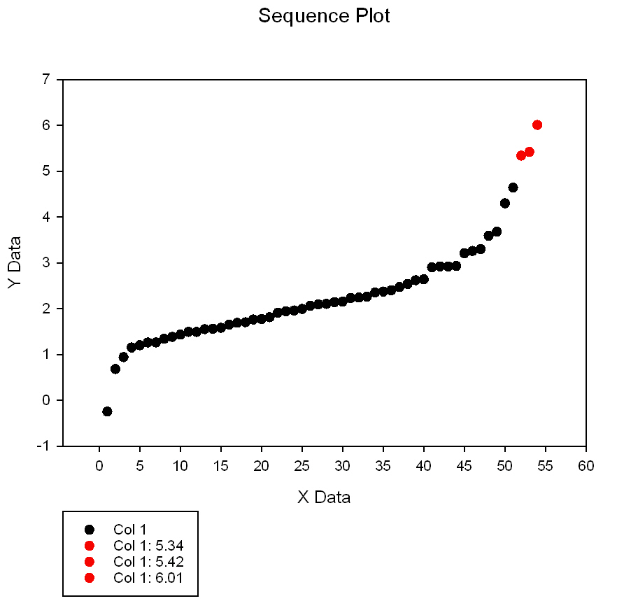
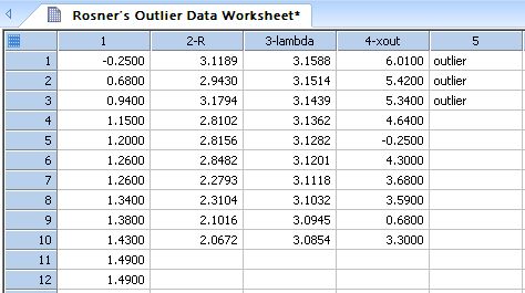
|
Rosner's Many-Outlier Test |
| This transform computes simple statistics rowwise * |
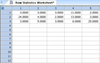
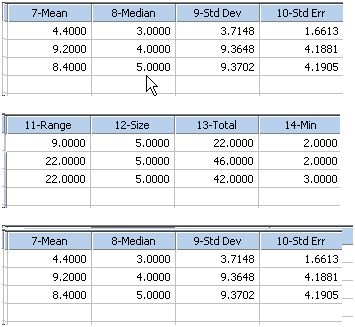
|
Row Statistics |
| Computes the sample cumulative distribution function of a column of data * |
|
Sample Cumulative Distribution Function |
| Savitzky-Golay Smoothing & Derivatives * |
|
Savitsky-Golay Filter |
| Plotting 2D-Implicit Equations as a Scatter Plot * |
|
Scatter Plot-2D Implicit Equation |
| Smooth Color Shade Transition from a Data Column |
|
Smooth Color Transition |
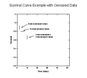
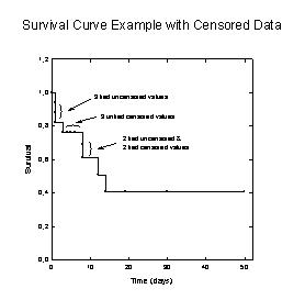
| Kaplan-Meier Survival Curves with Censored Data |
|
Survival |
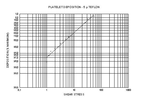
| Transform for the User Defined Y Axis Scale |
|
User Defined Axis Scale |
| This transform uses the Delta Method to estimate the variance (and standard error) of a function of the best-fit parameters in a regression model. * |
|
Variance of Functions of Parameters |
| Given a field of vector x,y positions, angles and lengths (in four columns), this transform will generate six columns of data ... |

|
Vector |
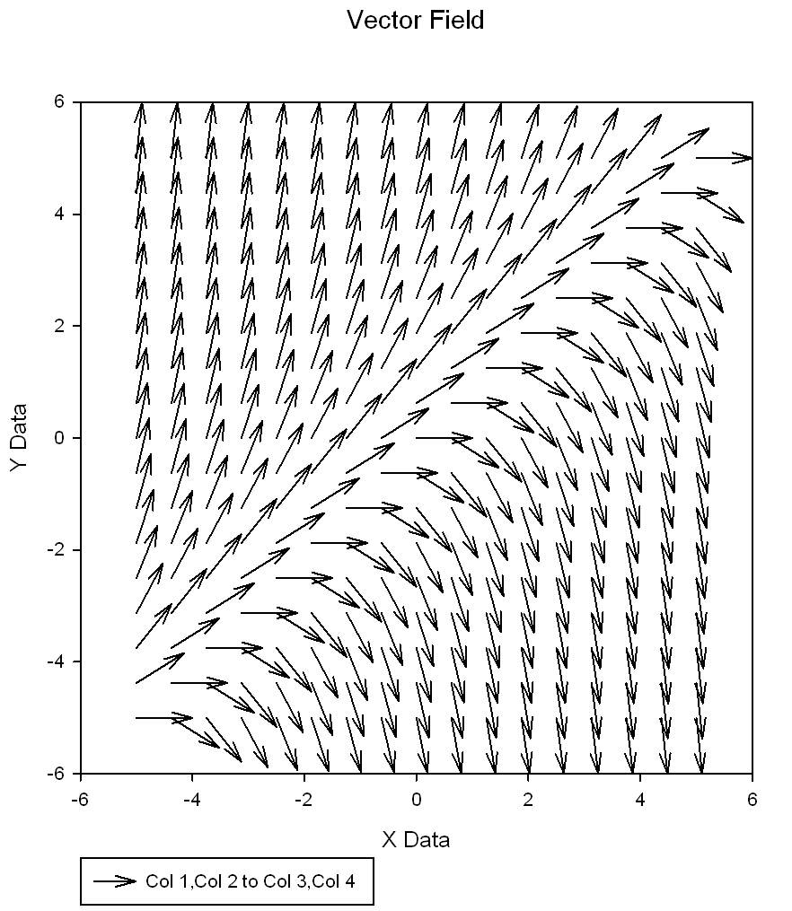
| This transform generates sampled data of a 2-dimensional vector field which can be used to create a vector plot using the XYXY data format * |
|
Vector Field Graph Data |
| Plotting 2D-Implicit Equations as Vector Fields * |
|
Vector Plot-2D Implicit Equation |
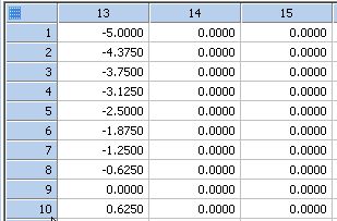
| Transform to Convert XY Many Z to XYZ Format * |
|
XY Many Z to XYZ Triplet Format |
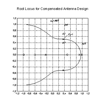
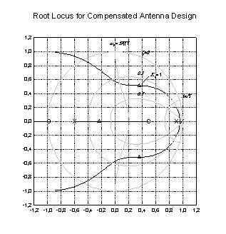
| Transform for z-Plane Design Curves |
|
Z Plane |
| Notebook Section - Transform Comments |
|---|
|
3D Histogram
↑
TOC
↓
3D Histogram * 

' 3D Histogram ' ' Enter data in two columns x, y ' Specify x,y column numbers xc, yc ' Specify x,y histogram intervals nx, ny ' Specify first column for results res ' Results are in x,y many z format ' x in col res ' y in col res+1 ' z1 to zny in cols res+2 to res+ny+1 |
|
3-Way ANOVA Cell Data
↑
TOC
↓
Converts indexed data for a 3-Way ANOVA design into a raw data format * 

'Converts indexed data for a 3-Way ANOVA design into a raw data format 'where the data for each ANOVA cell (a combination of factor levels) is 'output into a column of the worksheet. Each output column consists of the 'names of the factor levels followed by the data. If you have a m x n x p 'design, there will be m*n*p output columns. |
|
Akaike Information Criteria
↑
TOC
↓
Akaike Information Criteria - Model Comparisons * 

' Akaike Information Criteria - Model Comparisons ' For use with the output of the Nonlinear Regression Wizard ' Select regression Numeric Output Options to place parameters and residuals into the worksheet ' Specify the column numbers in Input for these output results |
|
Akaike Weights
↑
TOC
↓
Akaike Model Probabilities * 

'Akaike Model Probabilities ' put AICc values from your different regression models in a column with no missing values |
|
Area Under Curve
↑
TOC
↓
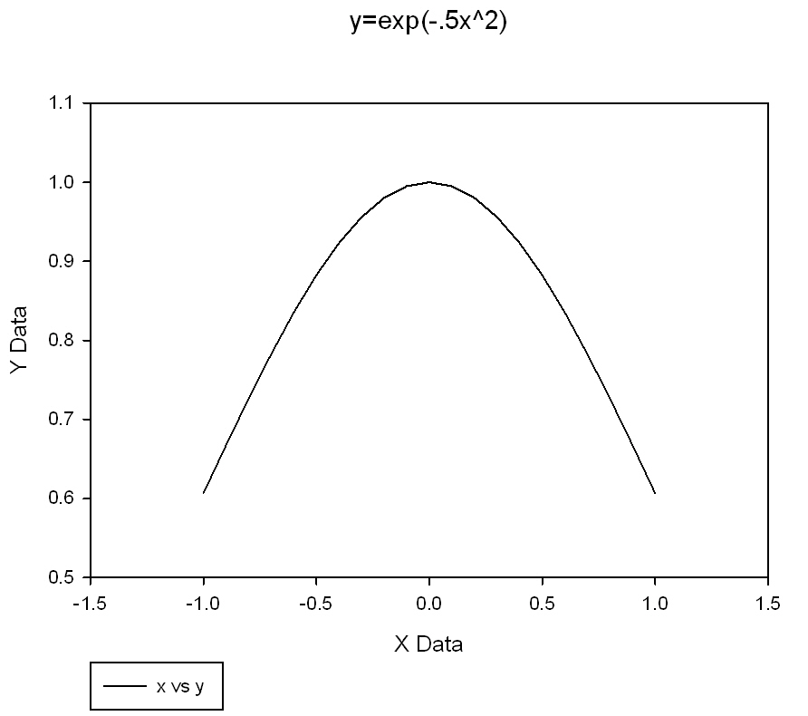
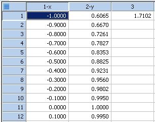
Transform for Calculating Area Beneath a Curve 

'*Transform for Calculating Area Beneath a Curve*

' This transform integrates under curves using the
'   trapezoidal rule  This can be used for equal
'   or unequally spaced x values

'   The algorithm is: sigma i from 0 to n-1; or
'   {yi(xi+1 - xi) + (1/2)(yi+1 - yi)(xi+1 - xi)}

' Place you x data in x_col and y data in y_col or
' change the column numbers to suit your data
' Results are placed in column res
|
|
Bivariate Data Analysis
↑
TOC
↓
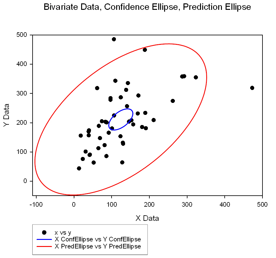
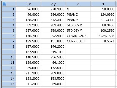
Transform to Compute Bivariate Statistics 

;*** Transform to Compute Bivariate Statistics *** ; This transform takes x and y data and returns ; the means, standard deviations, covariance (sxy), and ; correlation coefficient (rxy). You also have the option to compute ; graph data for the confidence ellipse of the mean and the prediction ellipse ; for adding a new observation which can also be used to identify outliers. ;If you want graph data created for the ellipses, you must select ;Radians for the angular unit below. ; Place your x data in x_col and y data in y_col ; or change the column numbers to suit your data. ; Numeric results are placed in columns res and res+1 ;Graph data results are placed in columns res+2, res+3, res+4, res+5. |
|
Bootstrap Method
↑
TOC
↓
Bootstrapping to Estimate Variance of a Statistic * 

''Bootstrapping to Estimate Variance ''of a Statistic ''----------------------------------------------------------------- ''x is data sampled from some common distribution ''f(x) is a statistic computed from the data ''For example, f(x) may estimate some parameter ''of the distribution. ''We want to estimate the variance of f(x) ''In the example below, the statistic computed from ''the data is the sample coefficient of variation ''and the its variance is estimated. Users can ''replace this statistic to suit their needs. |
|
Bootstrap Samples
↑
TOC
↓
Creates a number of bootstrap samples (sampling with replacement) of a user-selected column of worksheet data * 

'Creates a number of bootstrap samples (sampling with replacement) of a 'user-selected column of worksheet data. The samples are placed in 'contiguous columns starting at a position specified by the user. Note that if 'original data set has n distinct values, then there are (2*n-1) choose (n-1) distinct 'bootstrap samples. |
|
Box-Muller Bivariate Normal Deviates
↑
TOC
↓
Box and Mullers Bivariate Normal Random Number Generator * 

'Box and Mullers Bivariate Normal Random Number Generator |
|
Bubble Plot Symbol Size
↑
TOC
↓
Symbol Size for Bubble Plot (Symbol Sizexfm) 

' Symbol Size for Bubble Plot (Symbol Sizexfm) ' This transform converts a data column ' into symbol diameters and normalizes ' the largest value to a user specified ' symbol size The area of the symbol ' is made proportional to the data value 'NOTE: This transform is based on measurement units: Inches. 'For Millimeters, append "* 25" to the transform line: col(co)=(maxdia/sqrt(max(col(ci))))*sqrt(col(ci)) * 25 |
|
Control Chart
↑
TOC
↓
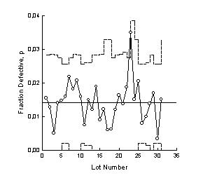
Transform for Fraction Defective Control Chart with Unequal Sample Sizes 

'Transform for Fraction Defective Control Chart 'with Unequal Sample Sizes ' This transform takes sample size and number of ' defectives returns the fraction of defectives ' and data for upper and lower control limit lines ' Place the sample size data in n_col and the ' number of defects in def_col; or change the ' column numbers to suit your data Fraction ' defective results are placed in the percent_col ' column; and the data for the control lines is ' placed in columns cl and cl+1,' |
|
Convert Cartesian To Polar
↑
TOC
↓
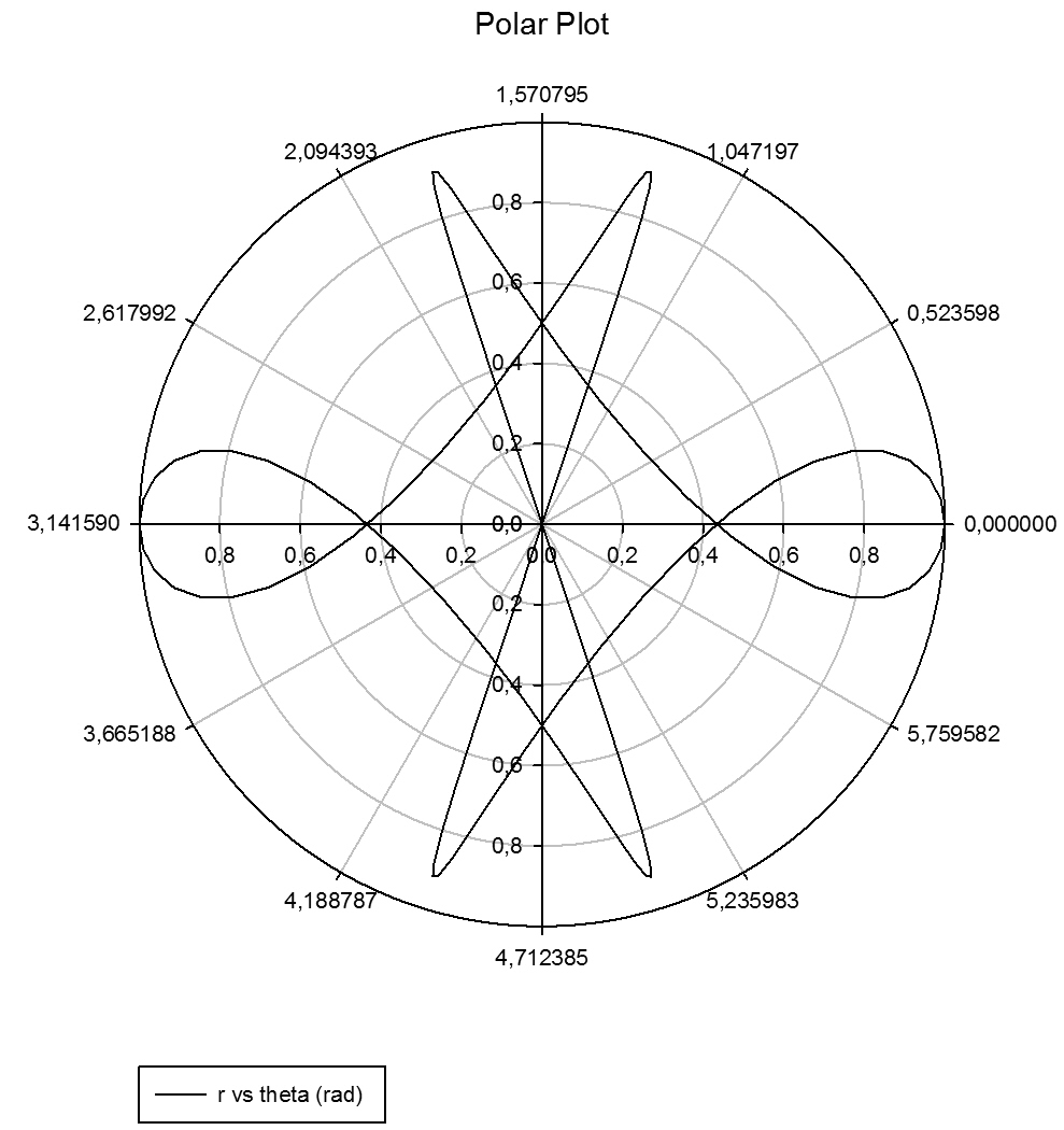
Convert data from Cartesian coordinates to Polar coordinates * 

'Convert data from Cartesian coordinates to Polar coordinates 'Make sure the Trigonometric units setting below is Radians. The 'following instructions use standard naming conventions for the 'coordinate systems. |
|
Convert Polar To Cartesian
↑
TOC
↓
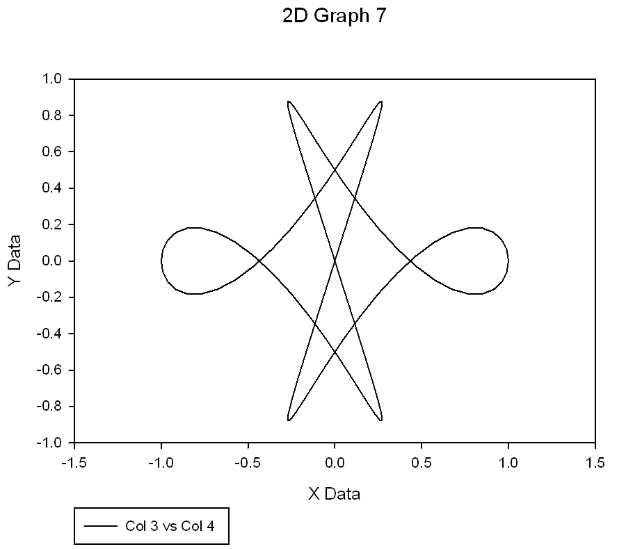
Convert data from Polar coordinates to Cartesian coordinates * 

'Convert data from Polar coordinates to Cartesian coordinates 'Make sure the Trigonometric units setting below is Radians. |
|
Convert Vector Plot Data Formats
↑
TOC
↓
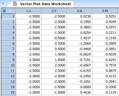
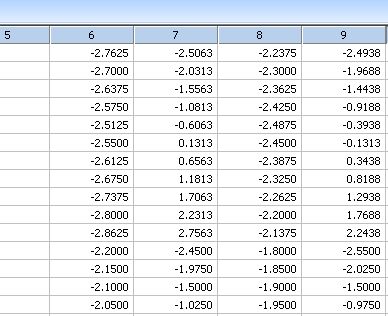
Vector Plot Conversion XYAM to XYXY * 

' Vector Plot Conversion XYAM to XYXY ' Given a field of vector x,y positions, angles ' and lengths (in four adjacent columns), this transform ' will generate four columns of XYXY data that ' corresponds to the XY locations of the beginning ' and end of the vector body. ' The input data is located in columns ci to ci+3 ' with x,y in columns ci and ci+1, vector angles (radians) ' in column ci+2 and vector lengths in column ci+3. ' The results are placed in columns co to co+3 |
|
Covariance_Correlation Matrix
↑
TOC
↓
Computes the sample covariance matrix or the sample correlation matrix of multivariate data * 

'Computes the sample covariance matrix or the sample 'correlation matrix of multivariate data. The output is a block 'of m columns and m rows, where m is the number of variables (columns) 'in the input data. The output begins at row 1 in the worksheet and the 'starting column of the output is specified by the user. The entry in the ith row 'and jth column of the output is the covariance or correlation of the ith and jth 'variables for the input data. |
|
Cubic Spline
↑
TOC
↓
Cubic Spline Interpolation and Computation of Derivatives 

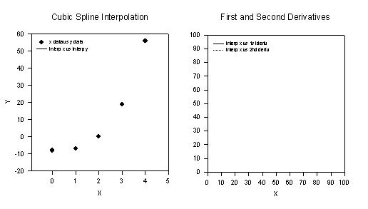
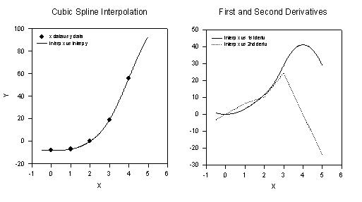
'**** Cubic Spline Interpolation and Computation **** ' **** of Derivatives **** 'This transform takes an x;y data set with increasing 'ordered x values and computes a cubic spline 'interpolation The first and second derivatives of 'the spline are also computed 'Two transform files are run in sequence This 'transform computes the spline coefficients The 'CBESPLN2,XFM transform computes the spline and two 'derivatives |
|
D'Agostino-Pearson Normality Test
↑
TOC
↓
D'Agostino-Pearson Normality Test * 

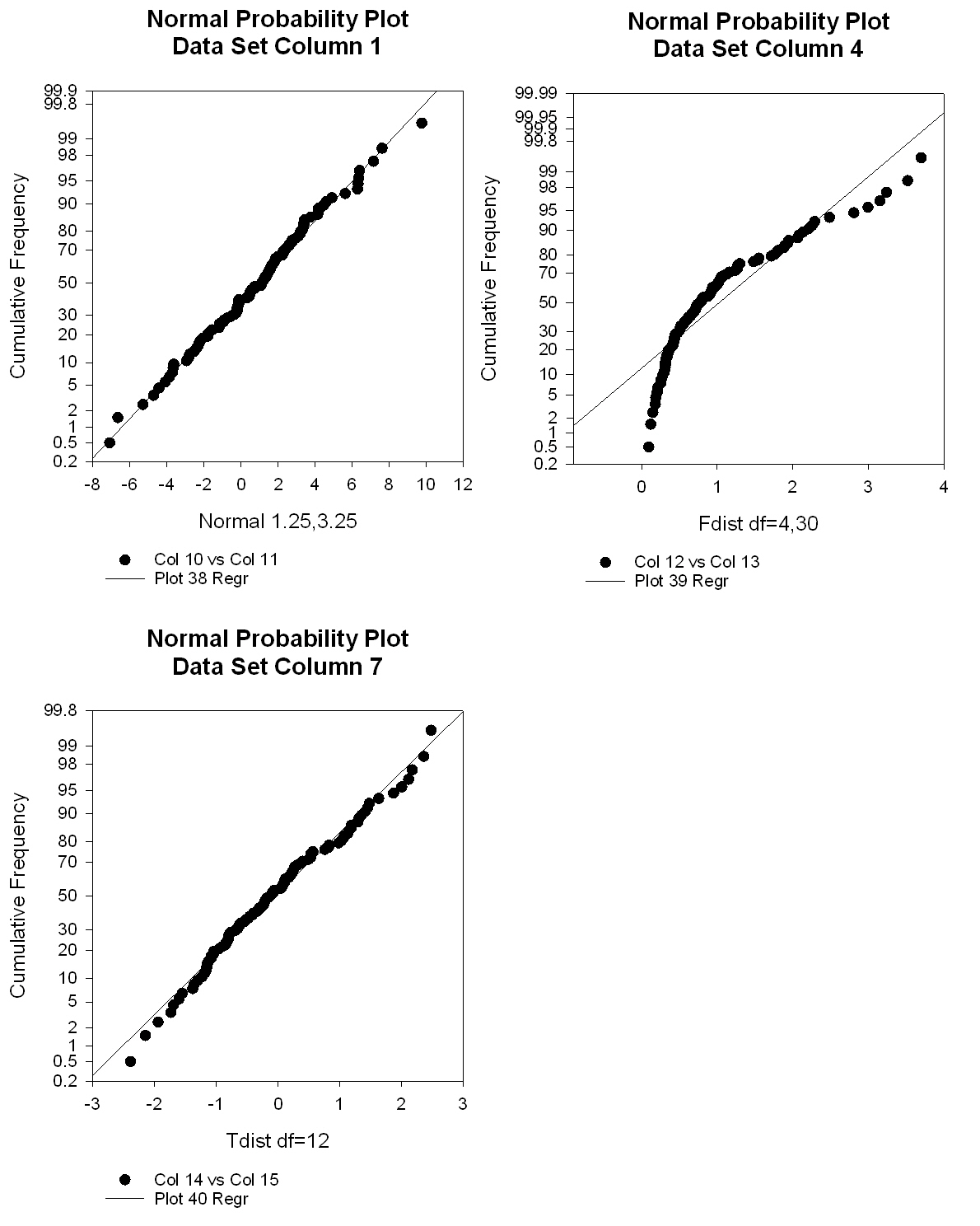
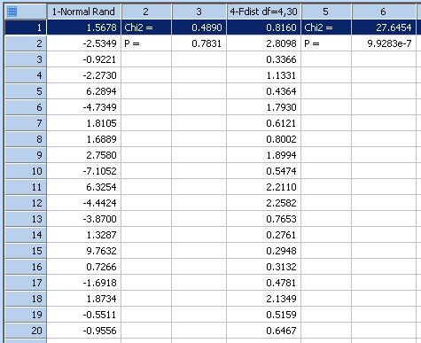
'D'Agostino-Pearson Normality Test 'A goodness-of-fit test to measure the departure of a data set from normality 'using estimates of skewness and kurotsis. This transform produces a 'Chi-square statistic and a P-value where the null hypothesis is that the data 'was sampled from a normal distribution. 'Enter the index of your input column to ci. Assign the output column to co. 'The sample size should be at least 8. |
|
Differential Equation - Runge Kutta
↑
TOC
↓
Solution of Coupled First Order Differential Equations by Fourth Order Runge-Kutta Method * 

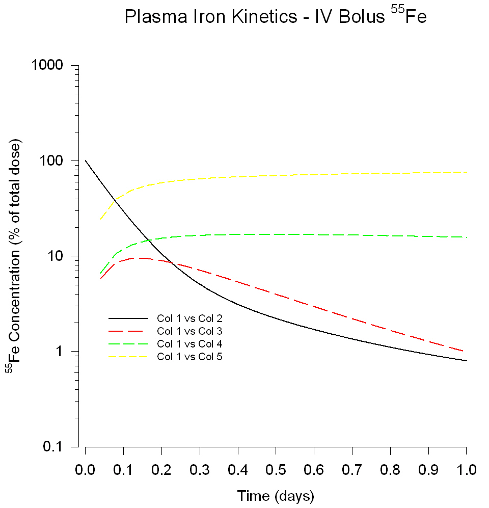
'*** Solution of Coupled First Order Differential *** '*** Equations by Fourth Order Runge-Kutta Method *** ' ***** Number of Equations ***** 'Enter the number of differential equations "neqn" 'the number of differential equations; less than or 'equal to 4 neqn = 4 'number of differential equations ' ***** Differential Equations ****** 'Set the functions fp1; fp2; fp3; fp4 to be equal to 'coupled first order ordinary differential equations 'where x is the independent variable and y1; y2; y3; 'and y4 are the dependent variables The number of 'equations must be equal to the neqn value set above 'If neqn < 4 then use zeros (0) for the unused 'equations |
|
Extrema Locator
↑
TOC
↓
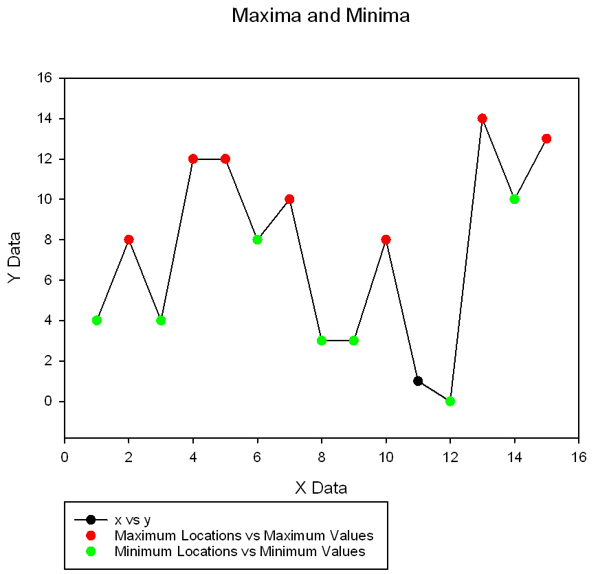
Procedure to locate all weak, local maxima or minima in a data set * 

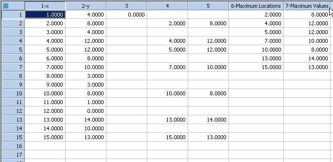
'Procedure to locate all weak, local maxima or minima in a data set. Weak means both sharp 'and flat peaks. This transform can be applied recursively to obtain a smaller set 'of more prominent extreme points. 'The user's raw data is specified by column indices XVarIndex for the independent 'variable and YVarIndex for the dependent variable. Be sure to enter an appropriate 'starting column for the output data so you don't override existing data. The output 'uses 5 consecutive columns if you don't remove low-level peaks and 9 columns if 'you do remove low-level peaks. 'A low-level peak (background noise) is defined as 'having a peak value less than some percent of the data range above the minimum. 'Maximum points are found by setting the mode to 1. Minimum points are found by 'setting the mode to -1. |
|
Frequency Plot
↑
TOC
↓
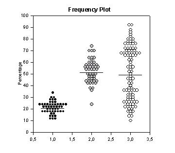
This transform creates frequency plots and mean bars of multiple y data columns 

' This transform creates frequency plots and mean bars of multiple y data columns
' It uses data in the first columns of the worksheet and creates column pairs for graphing
'
' Procedure - Data Entry
'   1. TURN INSERT OFF
'   2. Enter y data groups into columns in the worksheet starting with column 1
'   3. Select a symbol diameter d (try 0.05 to 0.10 in)
'   4. Specify the x locations for the groups (1,2,3,... are typically used since ticks are usually labeled)
'       Important!  Make sure that the number of numbers in x={1,2,...} equals the number of y data columns
'   5. Enter the width of your graph wg in inches (double click on graph to determine its width)
'   6. Enter the x range of your graph (usually 1 + number of groups)
'   7. Enter the vertical data interval w into which data points will be grouped
'   8. Enter the first vertical data interval start value (e.g., 0 if the vertical range is 0 to 100)
'   9. Enter the horizontal distance fx between symbols (try 0.05, use negative value for overlap effect)
'  10. Specify ml=1 if you want mean lines computed and specify mean line width eml
'  11. Specify intvl=1, 2 or 3 to place the y data at the bottom, center or top of the vertical data interval
'
' Procedure - Graph
'  1. Create x,y scatter plots for the column pairs
'  2. If mean lines are computed create an x,y line plot with no symbols from the last two columns generated
|
|
F-Test
↑
TOC
↓
Compare Two Nonlinear Curve Fits with the F test 

'***** Compare Two Nonlinear Curve Fits ***** '***** with the F test ***** 'This transform uses the residuals from two 'curve fits of functions from the same family 'to determine if there is a significant 'improvement in the fit provided by the higher 'order fitting function 'The F statistic is computed and used to obtain 'an approximate P value |
|
Gain Filter Smoothing
↑
TOC
↓
Gain Filtering 

' Gain Filtering ' This transform filters data by removing frequency ' components with power spectral density magnitude ' less than a specified value |
|
Gaussian
↑
TOC
↓
Gaussian Cumulative Distribution Function 

'*** Gaussian Cumulative Distribution Function *** '************** (CDF) Transform *************** ' This transform takes x data and returns the ' results of a Gaussian Cumulative Distribution ' function ' Place your x data in x_col or change the column ' number to suit your data Results are placed in ' column res |
|
Grubbs' Single-Outlier Test
↑
TOC
↓
Grubbs' Single-Outlier Test ( Maximum Normed Residual Test) * 

'Grubbs' Single-Outlier Test ( Maximum Normed Residual Test) 'This procedure detects a single outlier in a univariate data set sampled from 'an approximately normally distributed population. The null hypothesis is no outliers. 'A significant result of the two-sided version supports the alternate hypothesis that 'either the maximum or minimum values in the data set are outliers. 'A significant result of the left or right sided versions supports the alternate hypothesis 'that the minimum or the maximum values, respectively, are outliers. 'In the Input section below, specify the type of test (alternateHypothesis = 0 for two-sided, 'alternateHypothesis = -1 for left-sided, alternateHypothesis = 1 for right-sided), the 'signficance level sigLevel, the column index of the data set ci. 'The column index co is the first of two adjsacent output columns consisting of the test 'statistic computed from the data, the critical value of this statistic, 'and the conclusion of whether an outlier is suspected. |
|
Histogram Gaussian
↑
TOC
↓
Transform for a Histogram with a Superimposed Gaussian Distribution 

'******* Transform for a Histogram with a ******* '****** Superimposed Gaussian Distribution ****** ' This transform can be used to create histogram ' values for a sample with a normal distribution ' and the data for a smooth Gaussian curve for the ' histogram ' Place your normally distributed sample data in ' x_col or change the column number to suit your ' data Results are placed in columns res through ' rc+3, |
|
Jackknife Method
↑
TOC
↓
Jackknife Method to Estimate Variance of a Statistic * 

''Jackknife Method to Estimate Variance ''of a Statistic ''----------------------------------------------------------------- ''x is data sampled from some common distribution ''f(x) is a statistic computed from the data ''For example, f(x) may estimate some parameter ''of the distribution. ''We want to estimate the variance of f(x) ''In the example below, the statistic computed from ''the data is the sample coefficient of variation ''and the its variance is estimated. Users can ''replace this statistic to suit their needs. |
|
Jackknife Method - Bias Corrected
↑
TOC
↓
Jackknife Method with Bias Correction to Estimate Variance of a Statistic * 

''Jackknife Method with Bias Correction to Estimate Variance ''of a Statistic ''----------------------------------------------------------------- ''x is data sampled from some common distribution ''f(x) is a statistic computed from the data ''For example, f(x) may estimate some parameter ''of the distribution. ''We want to estimate the variance of f(x) ''In the example below, the statistic computed from ''the data is the sample coefficient of variation ''and the its variance is estimated. Users can ''replace this statistic to suit their needs. |
|
Kernel Smoothing
↑
TOC
↓
This transform smooths data using kernel smoothing 

' Kernel Smoothing ' This transform smooths data using kernel smoothing |
|
Linear Regression
↑
TOC
↓
Transform to Compute a Linear Regression with Confidence & Prediction Intervals 

;*** Transform to Compute a Linear Regression *** ;**** with Confidence & Prediction Intervals **** ; Place you x data in x_col and y data in y_col or ; change the column numbers to suit your data. ; Results are placed in columns res through res+5. |
|
Lowess Smoothing
↑
TOC
↓
Lowess Smoothing Example 

'******Lowess Smoothing Example****** |
|
Low Pass Smoothing
↑
TOC
↓
Lowpass Smoothing Filter 

' Lowpass Smoothing Filter ' This transform computes the fft, eliminates specified high frequencies ' and computes the inverse fft |
|
Low Pass Filter
↑
TOC
↓
First Order Low Pass Recursive Filter 

;**** First Order Low Pass Recursive Filter **** ;This filter will smooth data by reducing ;frequency components above the half power point. ;It generates the filtered ouput y(i) from the ;data x(i). ;y(i) = a y(i-1) + (1 - a) x(i) ;where a is computed from the specified half power ;point fc. |
|
Mesh Plot
↑
TOC
↓
Transform to generate XYZ triplet data for Mesh Graph 

'* Transform to generate XYZ triplet data for Mesh Graph * '* This transform takes an X range and a Y range * '* and generates the xy grid intersections and * '* the z values for a user defined function. * |
|
Multiple Key Sort
↑
TOC
↓
Performs an in-place sort of a block of data in the worksheet with multiple key columns * 

'Performs an in-place sort of a block of data in the worksheet with 'multiple key columns. The transform assumes the data begins in 'the first row of the worksheet. 'Define the worksheet region to sort. 'Adjust these values to your needs. |
|
Normalized Histogram
↑
TOC
↓
Transform to Generate Normalized Histogram 

; ** Transform to Generate Normalized Histogram ** ; This transform normalizes a bar chart to unit ; area. Box locations are shifted since bars are ; drawn about their center points ; Place your sample data in x_col or change the ; column number to suit your data. Results are ; placed in columns res through res+1. |
|
One-Way Frequency Analysis
↑
TOC
↓
This transform will find the unique items in the input column and give the count or frequency of each item in the column * 

'This transform will find the unique items in the input column and 'give the count or frequency of each item in the column. Optionally, a 'frequency table will be created and a chi-square test will be performed 'to test the equality of frequencies. 'To protect existing data, the output columns should be empty |
|
Polynomial Roots
↑
TOC
↓
This transform computes the real roots (zeroes) of a polynomial with real coefficients. * 

'This transform computes the real roots (zeroes) of a polynomial with real coefficients. 'The polynomial is defined by listing its coefficients in a column of the worksheet, using 'the first row for the constant term and subsequent rows for the coefficients in order 'of increasing powers of the independent variable. 'In general, if you are looking at the roots of the polynomial: ' '- - - - - - - - - - - P(x)=a0 + a1*x + a2*x^2 + ... + aN*x^N- - - - - - - - - - - - - - - - - - - - - ' 'Then the column of coefficients appears as: ' a0 ' a1 ' a2 ' : ' aN 'The last entry aN must not be zero and N must be no greater than 1000. 'In the INPUT section below, CoeffIndx is the column index for the coefficients 'and OutIndex is the output column index for the roots. If only looking for one root, 'you can set searchintervals =1. If you want to find all roots, searchintervals must 'be set higher. The default may not be adequate especially if some roots are very 'close to each other or the degree of polynomial is large (the maximum degree is 1000). |
|
Power Spectral Density
↑
TOC
↓
This transform computes the power spectral density (psd) of the data in column ci and places it in column co 

' Power Spectral Density ' This transform computes the power spectral density (psd) of ' the data in column ci and places it in column co. ' If a nonzero sampling frequency fs is specified then a frequency ' axis is placed in column co with the psd in the next adjacent ' column. ' If han = 1 then a Hanning window is applied to the padded data. ' Set Trig Units to Radians |
|
R Squared
↑
TOC
↓
Transform to Compute R Square (Coefficient of Determination) for Non-linear Curve Fits 

;** Transform to Compute R Squared (Coefficient *** ;** of Determination) for Non-linear Curve Fits ** ; Place you observations in y_col and the fit (predicted) ; values in fit_col. If you're fit problem has fixed weights ; for each observation, place the weights in weight_col. ; Change the column numbers to suit your data. ; ; Results are placed in column res if there are no weights ; and in columns res and res+1 if weights are included. ; ;Corrected R Squared values are corrected for the mean of observations. ;Uncorrected R Squared values remove this mean correction. |
|
Random numbers, Assorted Distributions
↑
TOC
↓
Generates random numbers with a given distribution determined by the user. 

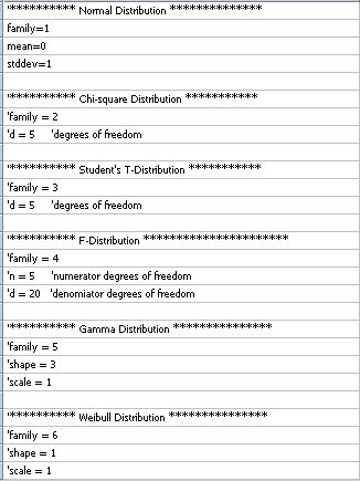
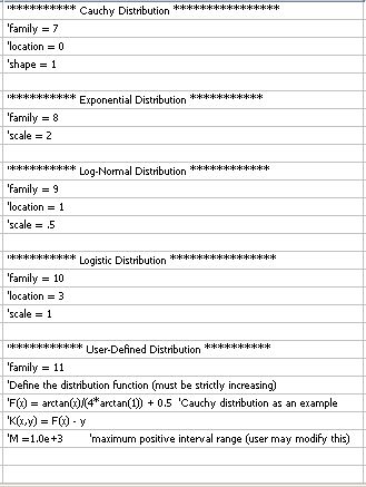
'Generates random numbers with a given distribution 'determined by the user. 'To use, set the number of samples and the output column 'below. Find your distribution in the list below 'and uncomment the statements defining the "family" 'and the distribution parameters. Modify the parameter 'values to suit your needs. Do not modify the value of '"family". Make sure you only remove the comments 'of the distribution you want to use. By default, 'we have selected the normal (Gaussian) distribution. |
|
Ribbon Plot Data
↑
TOC
↓
This transform takes x,y and multiple z columns and creates x,y,z ribbon triplets 

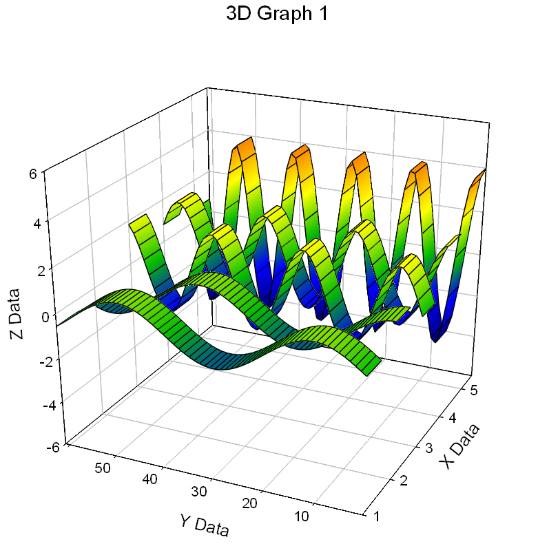
' Ribbon Transform (ribbon.xfm) ' This transform takes x,y and multiple z columns ' and creates x,y,z ribbon triplets ' Input Procedure ' 1. specify ribbon direction (yrib=1 creates ribbons that ' vary along y with an x width = width) ' 2. specify ribbon width (width) ' 3. specify starting column for data block (c1) ' 4. specify ncol the number of ribbons (z columns) ' The data block consists of an x column a y column and n z ' columns. As an example, the data block for 'y ribbons' consists ' of the x column which contains the x values for each ribbon and ' will have as many values as there are ribbons, the ' y column which contains the y values for the data along each ' ribbon, and n z columns which define the z values (height) for ' the n ribbons. ' Graph Creation Procedure ' 1. Select Mesh, XYZ triplet ' 2. For each ribbon repetitively highlight the XYZ triplet ' data columns and select Next. |
|
Rosner's Many-Outlier Test
↑
TOC
↓
Rosner's Generalized ESD Multiple Outlier Procedure * 

'Rosner's Generalized ESD Multiple Outlier Procedure 'This procedure detects up to 10 outliers in a univariate data set 'of size at least 25 sampled from an approximately normally distributed population. 'In the Input section you specify the index ci of the input data column 'and the index co of the first of four adjacent output columns. 'The column index cw specifies the first of three adjacent 'columns used as the workspace for computations. 'see "Quality control of semi-continuous mobility size-fractionated 'particle number concentration data. RC Yu, et al." article |
|
Row Statistics
↑
TOC
↓
This transform computes simple statistics rowwise * 

' Rowwise Statistics ' This transform computes simple statistics rowwise ' rowwise mean, standard deviation, standard error, range, size, ' total, min, max, missing and sum of squares are placed in the ' worksheet starting in column res |
|
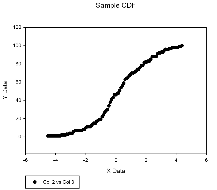
Sample Cumulative Distribution Function
↑
TOC
↓
Computes the sample cumulative distribution function of a column of data * 

'Computes the sample cumulative distribution 'function of a column of data |
|
Savitsky-Golay Filter
↑
TOC
↓
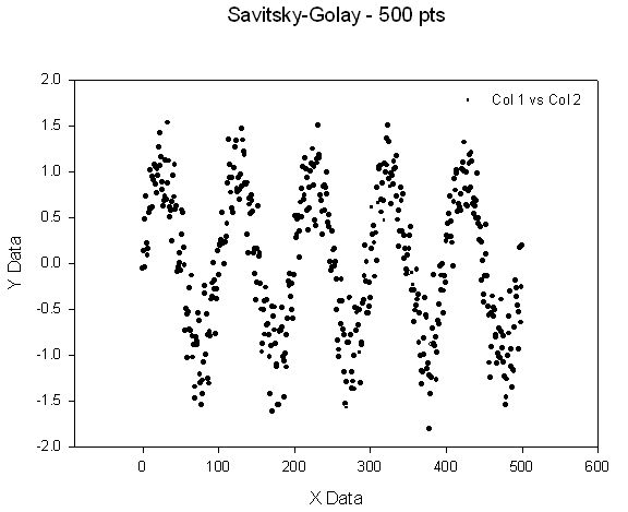
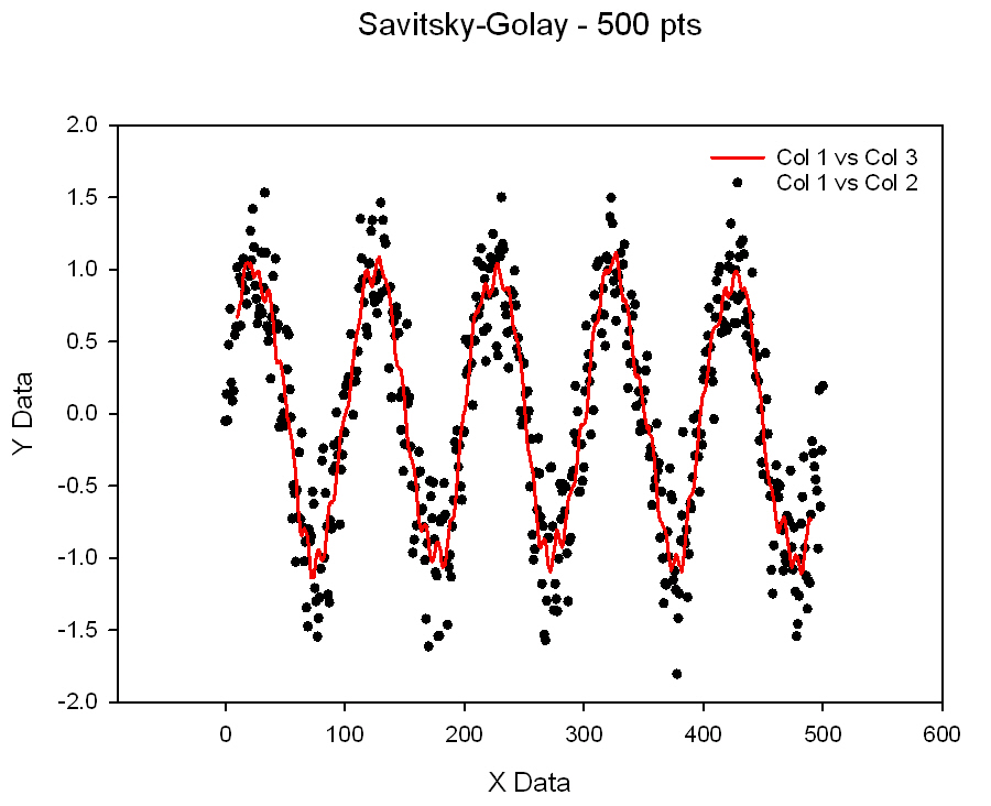
Savitzky-Golay Smoothing & Derivatives * 

' Savitzky-Golay Smoothing & Derivatives ' This is a moving average filter which tends to preserve ' peak characteristics - position, area, width. ' It uses m data points on either side of the current point for smoothing. ' Thus the filter length is 2m+1 and m points in the smoothed results will ' be skipped at the beginning and end of the data. ' Filter orders 2, 4 and 6 may be selected which corresponds to using a ' 2nd, 4th or 6th order polynomial in the smoothing. ' First and second order derivatives are computed using only the 2nd order filter. ' The x data is assumed to have equal intervals and be sorted. Only the y data is ' used in the analysis. ' The output is smoothed y, first derivative of smoothed y and second derivative of ' smoothed y and is placed in cols cout, cout+1 and cout+2. ' Three columns of temporary data are used in columns ctemp, ctemp+1 and ctemp+2. |
|
Scatter Plot-2D Implicit Equation
↑
TOC
↓
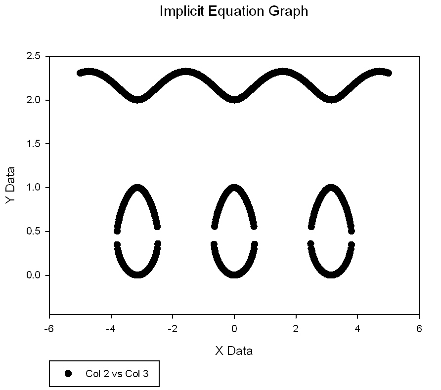
Plotting 2D-Implicit Equations as a Scatter Plot * 

'Plotting 2D-Implicit Equations as a Scatter Plot 'Define the function F for graphing the equation F(y,x)=0 F(u,v)=sin(v)^2 - u*(u-1)*(u-2) 'an example 'Below is the x-data and parameters to generate the graph data 'Adjust the three parameters ymin, ymax, minsep to suit your equations 'If you are uncertain, make the range from ymin to ymax large. 'minsep is the percent of this range that you expect y-values to be closest for any given 'x-value. 'The graph data will consists of two columns in the XY Pair data format for scatter plots. |
|
Smooth Color Transition
↑
TOC
↓
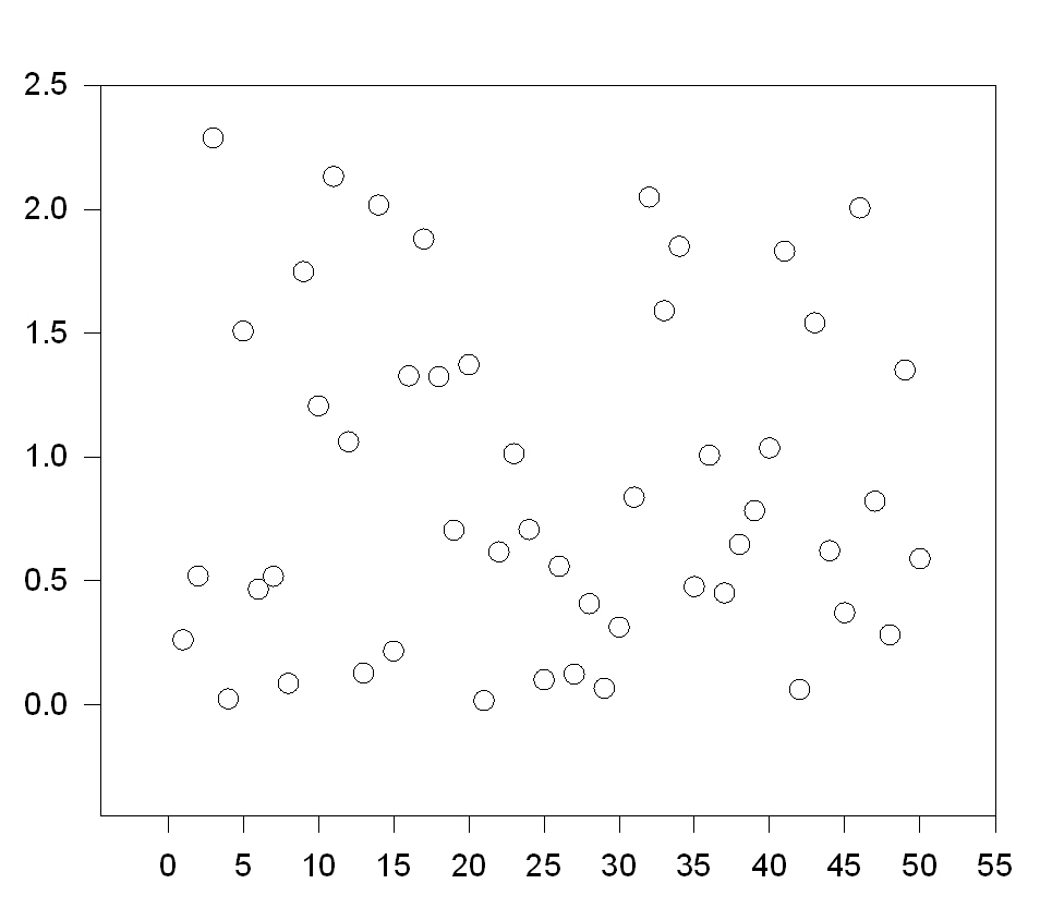
Smooth Color Shade Transition from a Data Column 

' Smooth Color Shade Transition from a Data Column ' This transform creates a column of colors which ' change smoothly from a user defined initial ' intensity to a final intensity as the data ' changes from its minimum value to its maximum ' value. |
|
Survival
↑
TOC
↓
Kaplan-Meier Survival Curves with Censored Data 

'*Kaplan-Meier Survival Curves with Censored Data* ' This transform calculates cumulative survival ' probabilities and their standard errors ' Enter survival times in column sur_col and a ' censor index in column cen_col (0=censored, ' 1=not), or change the column numbers to suit ' your data. Results are placed in columns res ' and res+1. ' Procedure: ' 1) sort by increasing survival time ' 2) place censored data last if ties ' 3) run this transform ' 4) plot survival data as columns 3 vs 4, as ' a stepped line shape with symbols |
|
User Defined Axis Scale
↑
TOC
↓
Transform for the User Defined Y Axis Scale 

;** Transform for the User Defined Y Axis Scale ** ;************* f(y)=log(log(100/y)) ************** ; This transform is an example of how to transform ; your data to fit a custom axis scale, and to ; compute the grid line intervals for that scale ; Place your y data in y_col and the y tick mark ; locations in tick_col or change the column ; number to suit your data. Results are placed ; beginning in column res |
|
Variance of Functions of Parameters
↑
TOC
↓
This transform uses the Delta Method to estimate the variance (and standard error) of a function of the best-fit parameters in a regression model. * 

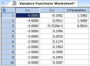
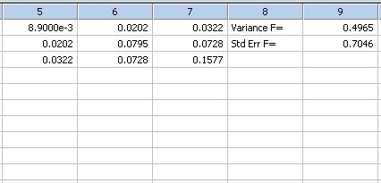
'This transform uses the Delta Method to estimate the variance (and standard error) of 'a function of the best-fit parameters in a regression model. 'The function is specified by the user. The input data consists of the parameter 'values and the covariance matrix of the parameters. The parameter values are output in the 'worksheet from the Regression Wizard. The covariance matrix is obtained by copying to the 'worksheet the covariance matrix in the Regression Wizard report. |
|
Vector
↑
TOC
↓
Given a field of vector x,y positions, angles and lengths (in four columns), this transform will generate six columns of data ... 

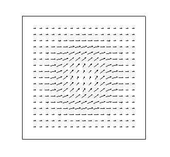
' ******** VECTOR PLOT TRANSFORM ******** ' Given a field of vector x,y positions, angles ' and lengths (in four columns), this transform ' will generate six columns of data that can be ' plotted to display the original data as vectors ' with arrow heads. ' The input data is located in columns xc to xc+3 ' with x,y in columns xc and xc+1, vector angles ' in column xc+2 and vector lengths in column xc+3. ' The results are placed in columns xc+4 to xc+9 ' To generate the vector plot, make a Line Plot ' with Multiple Straight Lines using XYpairs of ' these columns: xc+4 vs xc+5, xc+6 vs xc+7, ' xc+8 vs xc+9. ' This transform may be used in conjunction with the ' MESH.XFM transform which generates x,y pairs and ' corresponding z values. |
|
Vector Field Graph Data
↑
TOC
↓
This transform generates sampled data of a 2-dimensional vector field which can be used to create a vector plot using the XYXY data format * 

'This transform generates sampled data of a 2-dimensional vector field which 'can be used to create a vector plot using the XYXY data format. 'The vector field is defined by a pair of functions (F(x,y), G(x,y)) of cartesian 'coordinates x and y. This pair defines a vector whose initial point in the xy-plane 'is given by (x,y) and whose endpoint is at (F(x,y), G(x,y)) relative to this initial point. 'For the XYXY data format, the initial points are (x,y), which are specified on a 'rectangular grid, and the endpoints are (x+F(x,y), y+G(x,y)). |
|
Vector Plot-2D Implicit Equation
↑
TOC
↓
Plotting 2D-Implicit Equations as Vector Fields * 

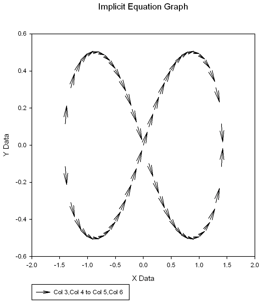
'Plotting 2D-Implicit Equations as Vector Fields 'Define the function F for graphing the equation F(y,x)=0 F(u,v) = (u^2+v^2)^2-2*(v^2-u^2) 'Below is the x-data and parameters to generate the graph data 'Adjust the three parameters ymin, ymax, minsep to suit your equations 'If you are uncertain, make the range from ymin to ymax large. minsep 'is the percent of this range that you expect y-values to be closest for any given 'x-value. 'The graph data will consists of four columns in the XYXY data format for vector plots. |
|
XY Many Z to XYZ Triplet Format
↑
TOC
↓
Transform to Convert XY Many Z to XYZ Format * 

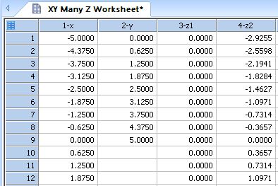
' Transform to Convert XY Many Z to XYZ Format 'The XY Many Z format has a layout with one X column, 'one Y column, a several adjacent Z columns. It provides a way 'of expressing data based on a rectangular grid in the XY-plane, 'where the number of Z columns equals the number of values in the 'Y column and each Z column has the same number of values as the 'X column. |
|
Z Plane
↑
TOC
↓
Transform for z-Plane Design Curves 

;****** Transform for z-Plane Design Curves ****** ; This transform generates the data for a unit ; circle and curves of constant damping ratio and ; natural frequency ; See Digital Control of Dynamic Systems, ; G.F. Franklin, J.D. Powell, pp. 32, 104. ; Root locus, zero and pole data is loaded from an ; external source |
 (ToolTip)